Getting Started

Installation

To install PICOcode, clone the git repository:

git clone https://github.com/picoexperiment/PICOcode.git

This downloads the repository as PICOcode under your current working directory and configures the copy for Git tracking. This clone can be made on your own computer or in your $HOME directory on a shared system like ComputeCanada (or both). Directions for each case follow.

Creating a virtual environment

It is common practice to create a virtual environment for python and install packages within it. This has several advantages, including keeping separate sets of installed packages in different environments, and saving you a huge headache later if something goes wrong with your python installation, since you can just delete the folder which contains the environment instead of having to purge and reinstall python.

To create a virtual environment, first download the virtualenv package by calling

pip install virtualenv

or pip3 install virtualenv if you have python 2 and 3 installed, e.g. on some versions of Ubuntu. Then, create a virtual evironment by calling

python -m virtualenv <path>

where <path> is the name of a new folder in which the environment will be created. Then, activate it by calling source <path>/bin/activate on Unix/Mac OS, or <path>Scriptsactivate.bat on Windows from the command prompt.

On your own computer

When the git clone download is complete you can install PICOcode and its dependencies with:

pip install -e PICOcode --user

The optional --user flag installs the packages in ~/.local/lib/; you may skip this if using a virtual environment. If you’d prefer a system-wide installation, you can run pip with root/admin privileges (e.g. prepend sudo). The optional -e flag installs the package in editable mode so that edits to the local code are automatically linked to the user’s python environment, and is recommended if you plan on developing.

On ComputeCanada

If you don’t yet have a ComputeCanada (CC) account linked to PICO, see docdb:4287 for instructions, including creating a python virtual environment.

When you’re able to ssh to graham.computecanada.ca you’ll find the PICO-60 and PICO-40L raw data grouped by runID under the PICO project directory: ~/projects/rrg-kenclark/pico/30l-16-data/ and ~/projects/rrg-kenclark/pico/40l-19-data/.

Detailed instructions for setting up your Python environment on CC can be found at the CC Python wiki page, but it should be sufficient to run the following:

module load python/3.7.7 scipy-stack/2020a

This loads the CC-provided Lmod modules for Python 3.7.7 and most of the packages required to use PICOcode into your current shell. This can be added to your ~/.bashrc to have it loaded automatically on each login. Keep in mind that non-interactive bash shells don’t source this file, so you’ll likely need to add this line to any CC bash scripts you write.

Finally, install PICOcode by running the following in the directory where you cloned the GitHub repository:

pip install -e PICOcode

At this point all PICOcode requirements should be satisfied, and the package should be ready to use.

Initial Setup

There are two files which may require some setup after installing PICOcode.

PICOcode.conf

The first time that PICOcode is imported, a config file is created in the user’s home directory depending on the system:

Linux/Mac OS	$HOME/.PICOcode.conf
Windows	C:Users<user>Documents.PICOcode.conf

This config file is structured as a JSON file containing two entries:

• ARCHIVE_DIR: the directory which contains raw PICO data, either in directories or as archives, in subfolders denoted by a data_series, i.e. raw data exists as <ARCHIVE_DIR>/<data_series>/<runID> or <ARCHIVE_DIR>/<data_series>/<runID>.tar

• SCRATCH_DIR, which contains extracted data if the runs are archived.

By default these point to the relevant locations on the Graham node of Compute Canada, which PICO uses for data processing. If you are using PICOcode on your own computer, you should edit this file to point to convenient directories.

librefprop

The NIST REFPROP program is used to compute various fluid properties, which is mainly used to calculate the Seitz threshold. The use of REFPROP (and its python wrapper ctREFPROP) depend on a file called librefprop, the format of which depends on the system in use.

Several versions have been compiled and are provided in PICOcode/REFPROP/lib. When first loaded, PICOcode will try each of these pre-compiled librefprop files until one works; if none of them do, it will throw an error. If this occurs, you may have to compile your own version (see instructions here). Please contact Colin if you are having issues with this.

Accessing PICO Data with PICOcode

PICO data comes in two forms: raw and reconstructed (a.k.a. recon). Raw data are generally time series of transducer data for a given run or event (e.g. pressure, temperature, acoustics, pictures), while recon data consists of processed raw data which is used to categorize events (e.g. pressure or Seitz threshold, AP to discriminate neutrons/alphas, Dytran to discriminate multiples).

Raw and reconstructed data are accessed using the Event and ReconFile classes. The use of these are described below.

The Event class

Note that the Event class is loaded to PICOcode’s namespace upon importing PICOcode, so it may be called with:

>>> PICOcode.Event(...).

This class is used to access raw data for individual PICO events. PICO data is stored with one directory per run, and one subdirectory per event (starting at 0, with up to 100 events per run), with some files related to run conditions stored in the run folder:

<runID>
├── <runID>.txt
├── DAQ30l_Setup.xml
├── DAQversion.txt
├── RunParameters.txt
├── 0
│   ├── Event.txt
│   ├── fastDAQ_0.bin
│   ├── fastDAQ_0_cal.txt
│   ├── PLClog.txt
│   ├── slowDAQ_0.txt
│   ├── temperature.txt
│   └── Images
│       ├── cam0_image30.png
│       ├── cam0_image31.png
│       ├── ...
│       ├── cam0_image70.png
│       ├── cam1_image30.png
│       ├── ...
│       └── cam3_image70.png
├── 1
│   └── ...
└── ...

PICO-40L, PICO-60, and some PICO-2L data are curently stored as archives on Compute Canada (CC) at:

Experiment Name	Data Series	Location on CC
PICO-40L	40l-19-data	/project/6007972/pico/40l-19-data
PICO-60	30l-16-data	/project/6007972/pico/30l-16-data
PICO-2L	2l-16-data	/project/6007972/pico/2l-16-data

The Event class is called by passing the full path to the run as the first argument, followed by the event number, followed by the name of the data to load as strings (either as a list, or as comma-separated values passed to *args). The requested data may include any or all of the following:

Load option	File location	Description of data
event	<run>/<event>/Event.txt	When the event began, trigger info, pressure setpoint, etc.
fastDAQ	<run>/<event>/fastDAQ_0.bin <run>/<event>/fastDAQ_1.bin <run>/<event>/fastDAQ_0_cal.txt <run>/<event>/fastDAQ_1_cal.txt	Data collected by the fastDAQ system. Includes signals from piezos, Dytrans.
slowDAQ	<run>/<event>/slowDAQ_0.txt	Data collected by the pressure cart PLC. Includes signals from pressure transducers, position transducers, valve states, DIO, etc. Similar data to PLC, but lower level and higher timing resolution.
temperature	<run>/<event>/temperature.txt	Data collected by the temperature PLC. Includes all RTDs, chiller setpoints, chiller loop flow data, humidity sensors.
PLC	<run>/<event>/PLClog.txt	Data collected over modbus from pressure cart. Lower timing resolution than slowDAQ, and contains some other info, e.g. PID values, sensor rms, etc.
DAQsettings	<run>/DAQ30l_Setup.xml	XML file containing run info from the DAQ VI. includes info such as setpoint, time spent compressed between events, pressure scan info (if used), etc.
rundata	<run>/<run>.txt	Text file containing all info from each events’ “Event.txt” file. Same info as the event option, but for all events in the run.
camdata	–	Currently Unimplemented.

Once the Event class has been loaded with one or more options, they are accessed via Event.<option>.<parameter>. For example, to access the data for PT4:

>>> event = PICOcode.Event("20200928_0", 24, 'slowDAQ')
>>> PT4 = event.slowDAQ.PT4

If working on a Graham node (a Compute Canada resource), or if you have altered your PICOcode.conf file appropriately, the path to the run directory may be substituted by the run ID only, and the Event class will search the locations contained in PICOcode.conf.

Example usage of the Event class

First, import PICOcode.

>>> import PICOcode

In this example, load fastDAQ, slowDAQ, and PLC data for the PICO-40L run 20200721_0 event 22.

>>> event = PICOcode.Event("20200721_0", 22, "fastDAQ", "slowDAQ", "PLC")
Loading  fastDAQ
Loading  slowDAQ
Loading  PLC

Load options may alternatively be passed as a list (for compatibility with old code). Use verbose=False to suppress info about loading data:

>>> event = PICOcode.Event("20200721_0", 22, ["fastDAQ", "slowDAQ", "PLC"], verbose=False)

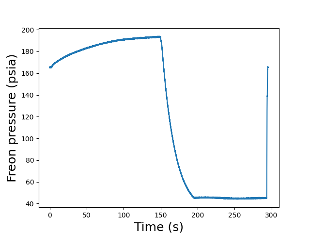
If we wanted to plot the pressure of the freon for this event versus time, we can use matplotlib:

>>> import matplotlib.pyplot as plt
>>> plt.plot( event.slowDAQ.elapsed_time, event.slowDAQ.PT4 )
>>> plt.show()

Which would produce the following plot (with some added elements):

The ReconFile class

Note that the ReconFile class is loaded to PICOcode’s namespace upon importing PICOcode, so it may be called with:

>>> PICOcode.ReconFile(...).

This class is used to access reconstructed PICO data, i.e. data that has been processed from its “raw” form. These data are stored in “recon files” located at /project/6007972/pico/recon/<branch>/<data-series>/output/, where <branch> is either current or devel, and <data-series> specifies the run series, e.g. 40l-19.

Within the recon output directory, each processed run has an associated recon folder containing its processed data. In addition, concatenated files exist in the output directory with data from all runs. The current list of processed files are:

File Prefix	Recon type	Data description
merged_all	2	Merged file containing data from all files.
merged_lvl1_xyz	2	Merged file with all data except XYZLookup
abub3hs	8	Pixel coordinates for bubbles in each event.
Dytran	1	Dytran info, t0, and fit parameters.
FastDAQ	1	Piezo info, t0, power, and AP parameters.
History	1	Pressure and temperature data at trigger, Seitz threshold, alarm conditions.
xyz_L1	2	Level one 3D reconstruction.
XYZLookup	2	Level two 3D reconstruction.

If the recon file being loaded is for a run (and it is located in output/<run>/), then the file prefix is appended with _<run>.txt. If the file is the concatenated file (located in output/), then the prefix is instead appended with _all.txt.

All data from recon files are loaded into numpy arrays. This is useful for making cuts; see the example below for how to do so.

Example usage of the ReconFile class

First, import PICOcode

>>> import PICOcode

An example of loading the merged_all file from the output directory in the current branch, then printing the freon pressure at the time of the trigger:

>>> recon = PICOcode.ReconFile("/project/6007972/pico/recon/current/40l-19/output/merged_all_all.txt")
>>> print(recon.PT4)
[45.95491 45.01076 52.85783 ... 56.51385 56.51385 45.03973]
>>> print(type(recon.PT4))
<class 'numpy.ndarray'>

Making a cut to scan for events at 35 psi, and which triggered within 1 PSI of the intended setpoint, then printing them one per line:

>>> cut = (recon.pset==35) & ( abs(recon.pset - recon.PT4) <= 1 )
>>> for run, ev in zip(recon.run[cut], recon.ev[cut]): print(run, ev)
20200107_3 0
20200107_3 1
20200107_3 2
20200107_3 3
20200107_3 4
20200107_3 5
20200109_0 0
...

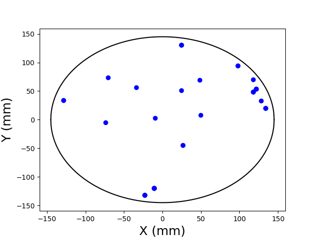
Update the cut to only include data after run 20200713_7 (this is the first run in which four cameras were recording data). Load the level two reconstruction, and plot X versus Y for events from the previous cut in which the bubble nucleated at least 5 mm from the wall (note this is ignoring the jar dome):

>>> cut = cut & (recon.run>"20200713_7")
>>> import matplotlib.pyplot as plt
>>> xyz = PICOcode.ReconFile("/project/6007972/pico/recon/current/40l-19/output/XYZLookup_all.txt")
>>> R = 145 # Outer jar radius, in mm
>>> for run, ev in zip(recon.run[cut], recon.ev[cut]):
...     xyzcut = (xyz.run==run) & (xyz.ev==ev)
...     if xyz.cR2[cut]**0.5 < R-5: plt.plot( xyz.cX[cut], xyz.cY[cut], 'ob' )

The above example would produce the following plot (with some added decoration):

Note that XYZLookup_all.txt should be merged into merged_all_all.txt, but this is not currently possible. In the future (when it is merged), the above example will not be useful.